The field map

app/Support/fieldmap.ts renders a field to SVG, server side, from the flight record. It is the site's main visual, and it is deliberately not an illustration: every marker is a row in detections, every orange cell is a row in the prescription's zones, and the boundary is the field's stored ring. Change the data and the picture changes.

That is the whole argument the page is making, so drawing it any other way would undercut it.

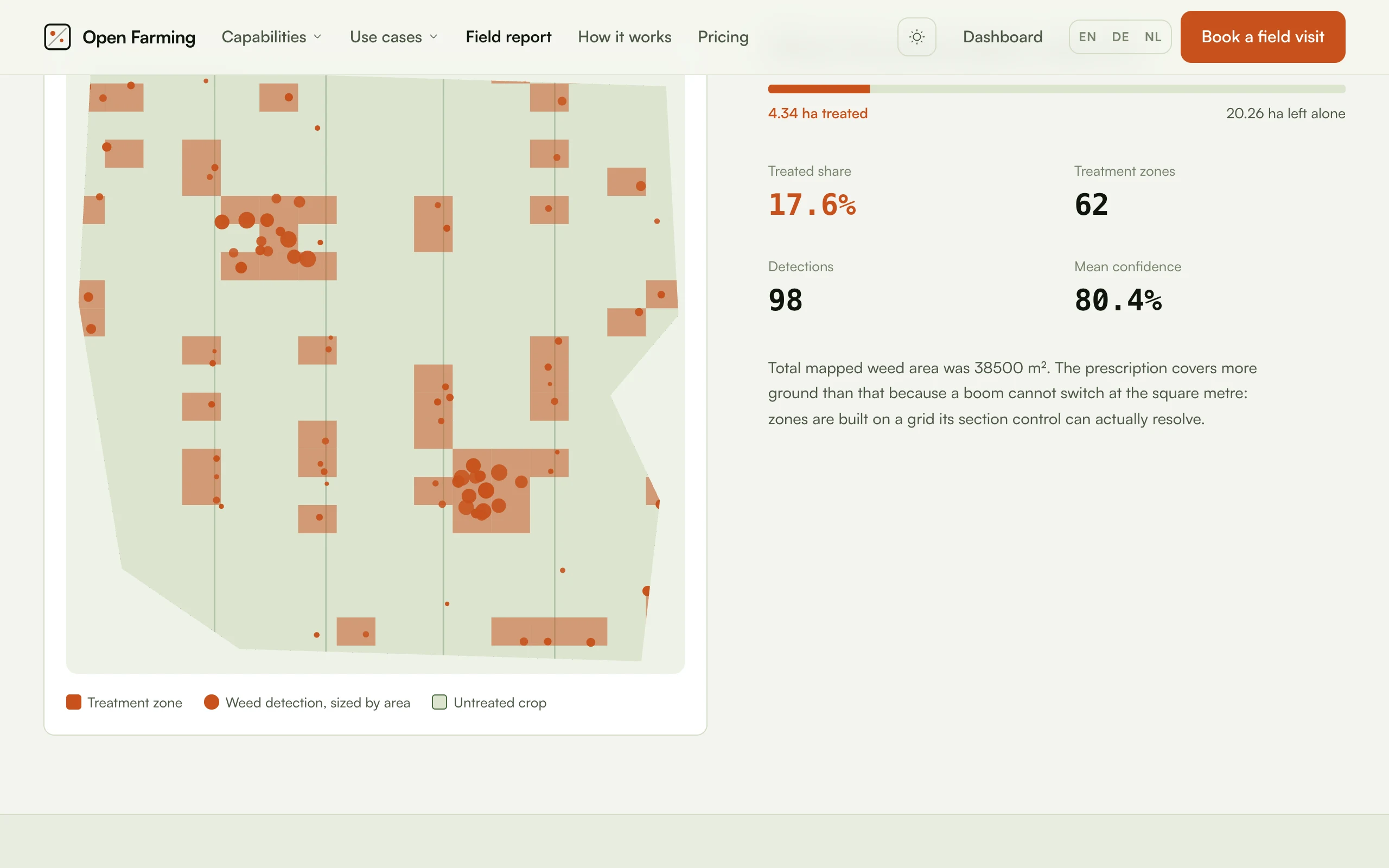
The map at full size on /field-report, with the figures beside it derived from the same records.

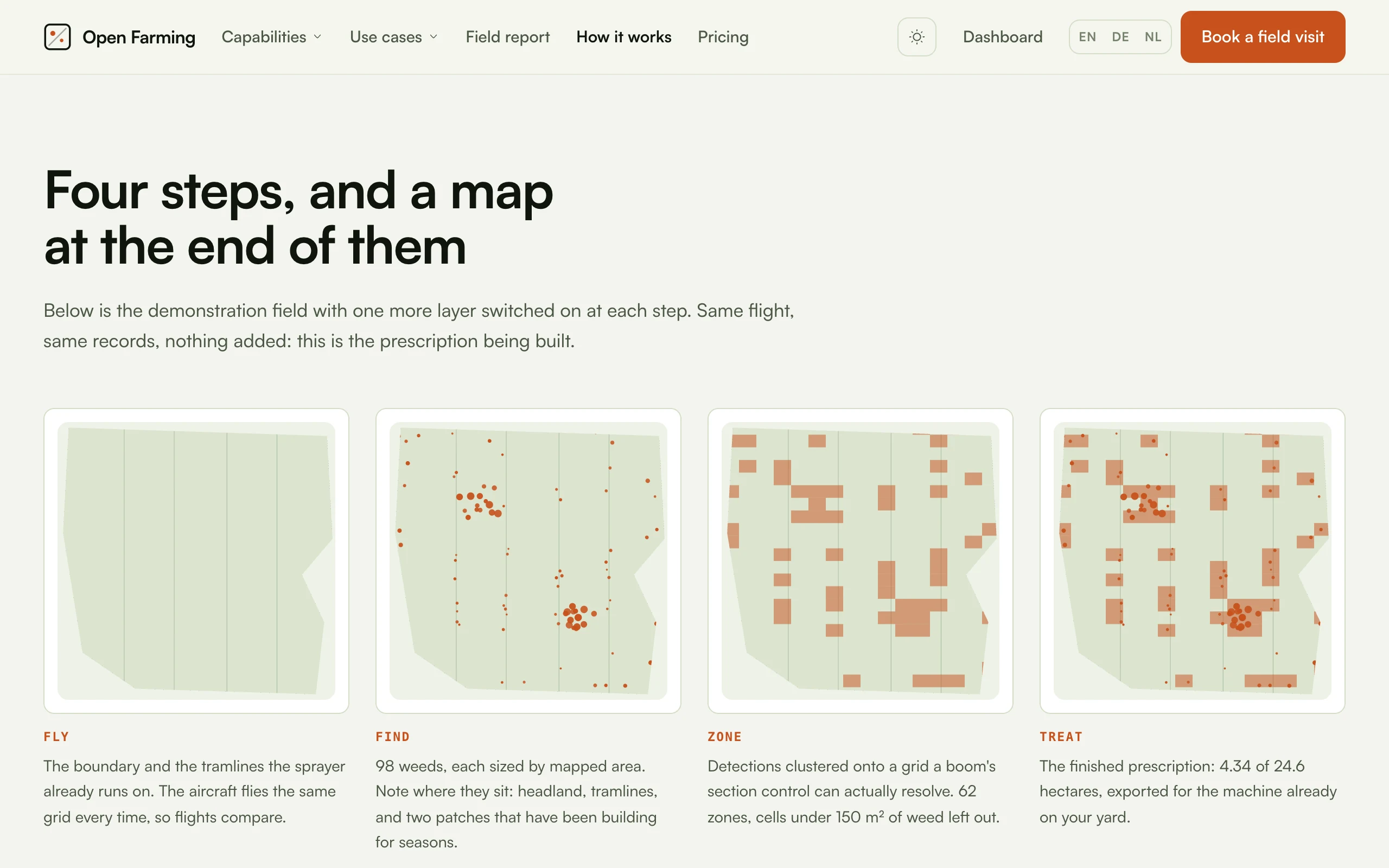
The /how-it-works page draws the same record four times, switching on one layer each time: the boundary and tramlines, the detections sized by mapped area, the clustering onto a grid, and the finished prescription. It is the clearest demonstration of what the options below actually control.

Why SVG, server side

The record already carries normalised 0..1 coordinates, so the SVG needs no projection and scales to any container. The viewBox is 0 0 1 1. There is no map library, no tile server and no client bundle involved in the main visual on the home page.

The API

renderFieldMap(report: FieldReport, options: FieldMapOptions): string
renderFieldMapSwitch(report: FieldReport, options: MapSwitchOptions): string
renderTreatedBar(report: FieldReport): string

title is required because the map carries real information, so it always needs a description. It is also hashed into the clipPath id and the radio group name, so two maps on one page cannot share a clip path or steer each other's switch.

Detail pages use subsets deliberately: a page arguing one point draws one layer.

Layer order

1. clipPath from the boundary ring
2. The boundary path itself, whose fill is the backdrop
3. Imagery, if requested and present
4. Tramlines
5. Zones
6. Detections

Imagery sits under the vectors because the picture is the ground and the vectors are what we found on it. Everything above the boundary is clipped to it, because a stitch always overflies the field and the neighbour's ground is not ours to publish.

Detection radius follows mapped area, sqrt(area_m2) / 2600, floored at 0.0035 and capped at 0.014 so a small detection stays visible and a large patch does not swamp its neighbours. Fill opacity carries confidence: 0.55 + confidence * 0.45.

Imagery, and why bounds matter

preserveAspectRatio="none" on the image layer is correct rather than lazy. An orthomosaic is already rectified to a rectangle of ground, and bounds says which rectangle, so stretching it to exactly that footprint is what puts a pixel over the square metre it was taken of. Letting it letterbox instead would shift every pixel away from the detection drawn on top of it.

A footprint with no area, or an inverted one, draws nothing. Showing no imagery is better than showing the field mirrored.

The plan and imagery switch

renderFieldMapSwitch puts two radios and a pair of labels over the map. It is CSS rather than a script: the map is server rendered from the flight record, and making the one control on it depend on JavaScript would be the only part of that page that does. Both states live in one SVG, so switching is a repaint with nothing to fetch and nothing to re-render.

With no imagery attached, renderFieldMapSwitch returns exactly renderFieldMap. No tabs, no empty state, no control that switches to a blank frame.

The imagery layer starts hidden and is revealed by CSS. A map that emits the layer without a switch over it would download an orthomosaic nobody can ever see, which is the whole page weight of the feature for none of its value. That is why showImagery defaults to false.

Default tab labels are translation tokens ({t:fieldReport.viewPlan}) rather than English, because the translation pass runs over the finished HTML and a view has no locale to hand at render time.

Attaching an orthomosaic

A mapping flight lands two things. The vectors are already published by catalog:sync. The other is the orthomosaic: every frame from the flight stitched and rectified into one picture of the whole field. Attaching it turns the map from a plan of the ground into the ground, with the same detections over it.

buddy imagery:attach ./lindenbach-2026-04-18.webp

buddy imagery:attach ./ortho.webp --bounds="-0.04,-0.03,1.05,1.02" --resolution 4

buddy imagery:attach https://cdn.example/ortho.webp --field lindenbach-nord

Note the equals sign. A leading minus is the ordinary case for a footprint, and --bounds -0.04,… would be read as a flag by any argument parser, this one included, so the value has to be attached to the option.

Omitting --bounds assumes the image covers the field exactly, which is almost never true of a real stitch.

A local file is copied into public/imagery/. A URL is stored as given.

Serve a derivative, not the master

The map ships the image inside the page, so a 400 MB GeoTIFF would be 400 MB on the wire. A few thousand pixels across is more than the map can show. Produce the web copy with the same tooling that made the stitch:

gdal_translate -of WEBP -outsize 3000 0 -co QUALITY=82 ortho.tif ortho-web.webp

See Ingest and photogrammetry for where the stitch comes from, and how to read the footprint out of the GeoTIFF rather than guessing it.

The treated bar

renderTreatedBar is deliberately not a progress bar with a filled track. It is a proportion of one field, so it is drawn as one bar split in two, with the split at the measured ratio: 17.6% on the demonstration field.