Targeted weed control
On this page 11
Spray the weeds, not the field
Cameras and on-board models find weeds plant by plant, then only the affected square metres get treated.
| Category | Act |
| Slug | targeted-weed-control |
| Cadence | Two to four scouting flights per crop, timed to the herbicide windows |
| Payload | RGB camera at 1 cm/px, downward LiDAR for canopy height, RTK |
| Needs a visit first | No |
The problem
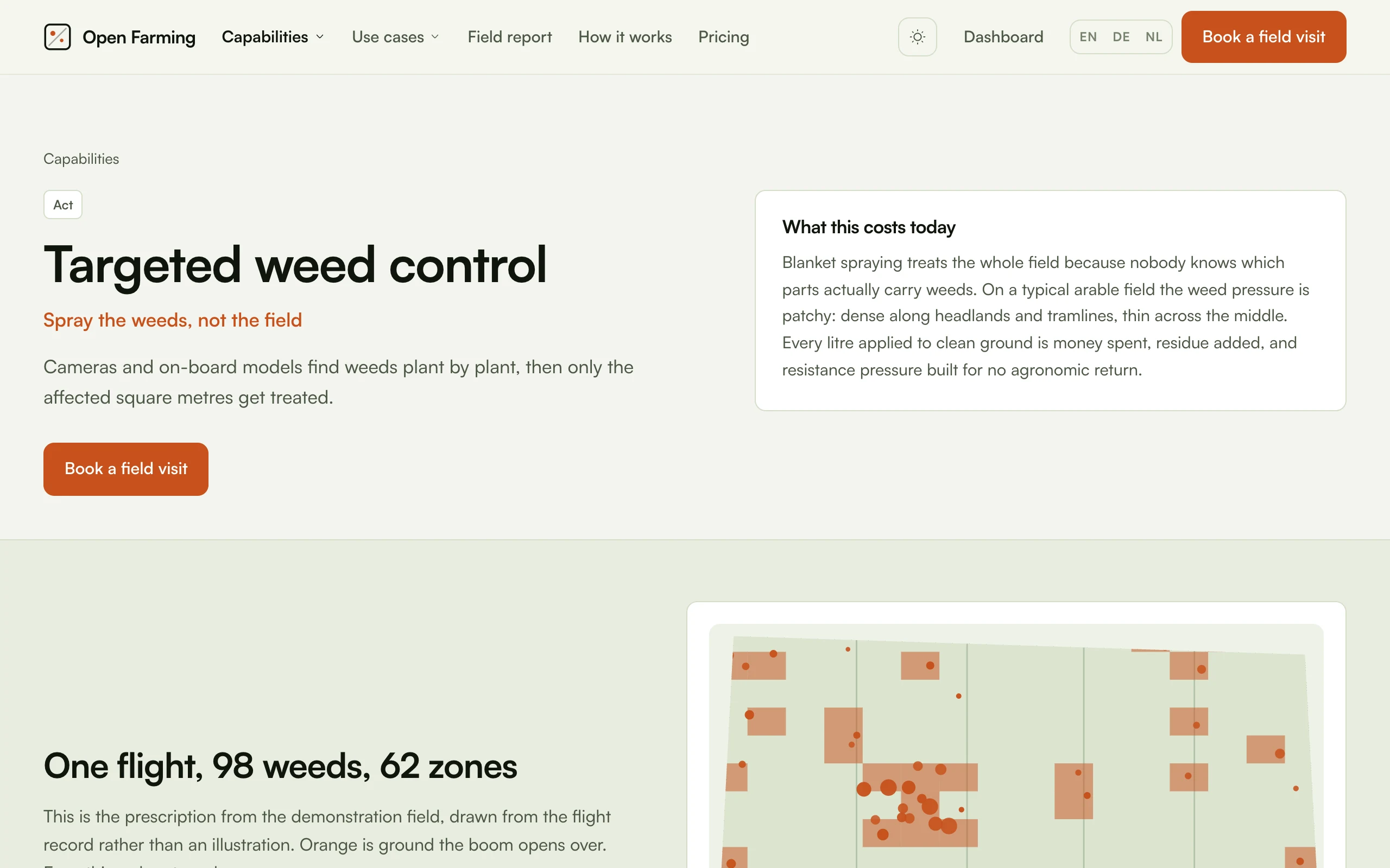
Blanket spraying treats the whole field because nobody knows which parts actually carry weeds. On a typical arable field the weed pressure is patchy: dense along headlands and tramlines, thin across the middle. Every litre applied to clean ground is money spent, residue added, and resistance pressure built for no agronomic return.
How it works
| Step | What happens |
|---|---|
| Scan | The drone flies a fixed grid at low altitude and photographs the canopy at centimetre resolution |
| Classify | An on-board model separates crop from weed and tags each detection with a species guess and a confidence score |
| Map | Detections are clustered into treatment zones and written to a prescription map with a buffer you set |
| Treat | The map loads into your section-control sprayer or spot-spray rig, which opens nozzles only over the marked zones |
The drone does not spray. In Germany and most of the EU, aerial application of plant protection products is prohibited by default under Pflanzenschutzgesetz §18, with narrow exemptions, most prominently steep vineyard terrain. The machine that is already permitted to treat the field is what treats it. See Regulation.
What you get
- Weed density map
- ISOXML or shapefile prescription
- Species breakdown per zone
- Before and after comparison
What the dashboard measures
- Treated area as a share of field area
- Product volume per hectare
- Detections by species
- Zone count and mean zone size
On the demonstration field: 98 detections, 62 zones, 4.34 of 24.6 hectares, which is 17.6%.
Where it matters most
Winter wheat, maize, sugar beet, organic farms, contractors.
Sugar beet is where it pays first: wide rows, slow early growth, an expensive repeated herbicide programme, and weeks of exposed soil.
Build it
This is the capability with the money in it and the one that needs real engineering. Build it third, after field mapping and something with a short pipeline.
Flight parameters
| Parameter | Value | Why |
|---|---|---|
| Ground resolution | 1 cm/px or better | Below that, a two-leaf blackgrass seedling is under two pixels |
| Altitude | 12 to 25 m AGL depending on lens | Which is why this flight covers far less ground per battery than a mapping flight |
| Overlap | 60% forward, 40% side | Enough to mosaic, not enough to need full photogrammetry |
| Timing | Still air, overcast or high sun, no long shadows | Shadow edges are the single biggest source of false positives |
| Coverage | 6 to 12 ha per battery | Plan two to four batteries per field |
Do not fly this at photogrammetry altitude and hope to upsample. The species call comes from leaf shape, and leaf shape needs pixels.
Hardware
| Item | Why | EU source | US source | Indicative |
|---|---|---|---|---|
| Airframe, 6 kg class | Slow, low, stable, 30 minutes | Holybro X500 V2 via Drone Parts Center | GetFPV | €400 to €700 |
| 24 to 60 MP camera, global or mechanical shutter | 1 cm/px at a sane altitude | Sony ILX-LR1 | B&H | €2,500 to €3,200 new |
| Budget camera | 1 cm/px at 15 m instead of 40 m | Raspberry Pi GS camera at BerryBase | Adafruit | €55 plus lens |
| RTK GNSS | Puts a detection on the right square metre, which is the whole point | ArduSimple simpleRTK2B | SparkFun | €200 to €300 |
| Height-hold rangefinder | Constant AGL over rolling ground keeps the scale constant | LightWare SF000/B or Benewake TFmini-S | RobotShop | €40 to €300 |
| Canopy LiDAR, optional | Canopy height separates crop from weed where colour cannot | Livox Mid-360 | RobotShop | €700 to €900 |
| On-board compute, optional | Only needed for real-time spot spraying, not for mapping | Jetson Orin Nano Super via Antratek | Seeed Studio | €250 to €900 |
In-house software
| Stage | What we run | Licence | Replaces |
|---|---|---|---|
| Detection model | RF-DETR or RT-DETR fine-tuned on our own labelled frames | Apache-2.0 | per-hectare weed mapping services |
| Alternative | MMDetection, torchvision, or Ultralytics YOLO | Apache-2.0 / AGPL-3.0 | |
| Tiled inference | SAHI sliced inference over full frames | MIT | |
| Labelling | CVAT or Label Studio | MIT / Apache-2.0 | Roboflow subscription |
| Georeferencing | Frame corners from RTK pose plus camera model, no full stitch needed | own code | |
| Clustering | Grid binning with an area threshold, then buffer and merge | own code | |
| Export | ISOXML TASKDATA and ESRI shapefile via GDAL/OGR | MIT | terminal vendor tooling |
| Serving | This repository's Detection and TreatmentMap models | MIT |
Ultralytics YOLO is AGPL-3.0. It is the easiest thing to reach for and the most expensive mistake to make in a commercial product, because the AGPL reaches your service, not just your binary. Either buy their commercial licence or start on an Apache-2.0 detector. See Perception models.
The clustering step, concretely
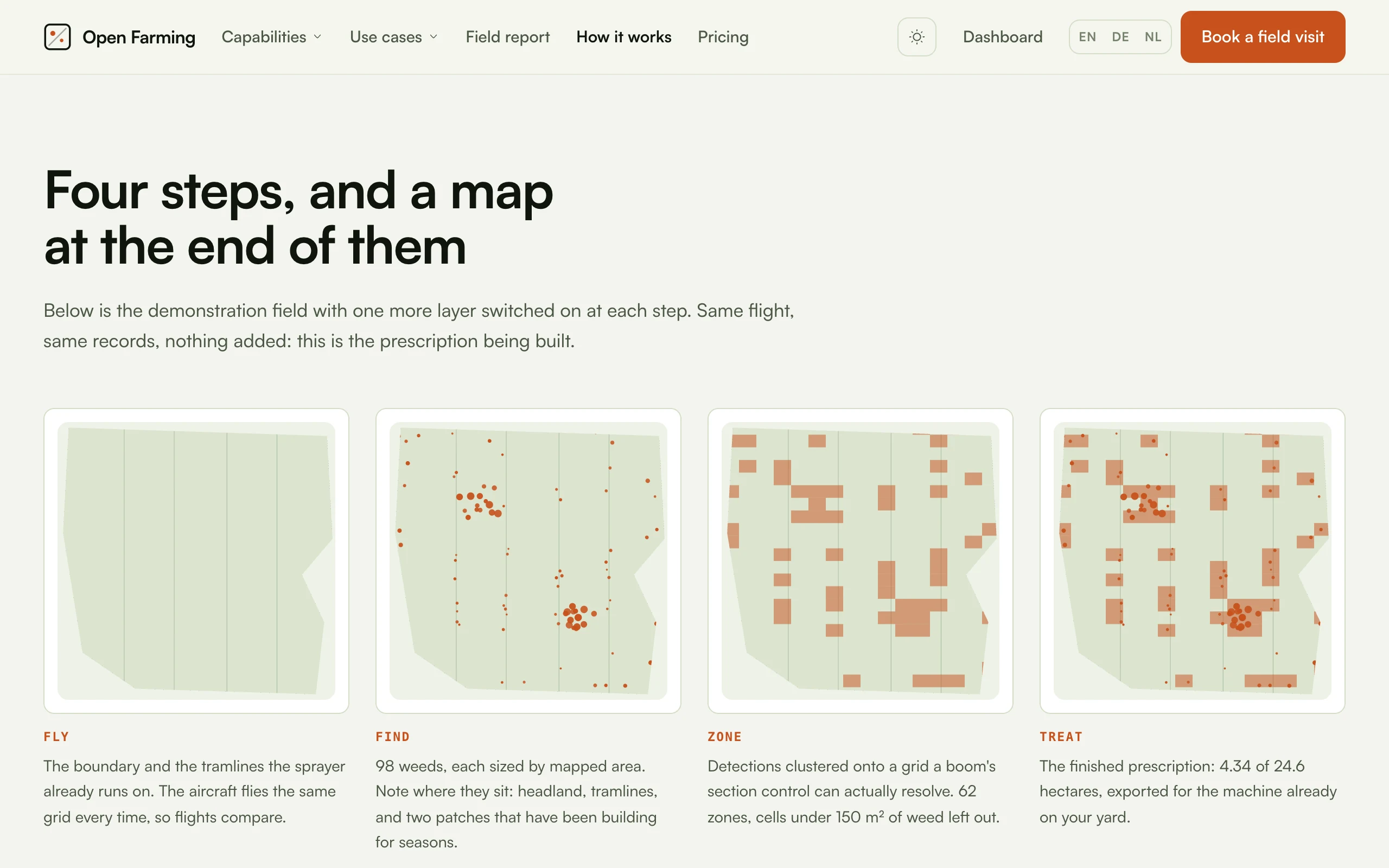
That is the clustering, drawn. Same flight record in all four frames, one more layer switched on each time.
This is the part everyone underestimates, and the part demo-field.ts
reproduces so the site's map is honest about it.
- Bin detections onto a grid whose cell is what your boom can actually resolve. On a 24 m boom with 8 sections, that is 3 m across. The demonstration field uses a 16 by 22 grid over 24.6 ha, which is about 700 m² per cell, roughly 31 by 23 m on a square block: a section-control prescription rather than a spot-spray one.
- Switch a cell on when the weed area inside it reaches a threshold. Below that, opening the nozzle is not worth the pass.
- Assign a rate by weight. The demonstration field uses 110, 140 and 180 l/ha.
- Buffer the live cells outward by the sprayer's positioning error plus the nozzle's spread, then merge adjacent cells.
A prescription finer than the machine can follow is a map no machine can follow. The buffer is where the agronomic argument lives: too small and you miss the plants at the edge of a patch, too large and the saving disappears. Make it a setting, and record what it was for every prescription.
Cost efficiency
- Label your own data, in your own fields. A public weed dataset trained on a different country's soil, camera and growth stage will disappoint you. Budget 2,000 to 5,000 labelled frames per crop for a first usable model. This is the real cost of the capability and it is one-off per crop, not per hectare.
- Skip on-board inference at first. For a prescription that gets loaded before the next pass, processing on the ground within the hour is fine and removes a whole class of hardware and thermal problems. Add a Jetson when you do real-time spot spraying.
- Use the free satellite layer to target the flight. A Sentinel-2 pass from the Copernicus Data Space is free and tells you which fields have a problem worth flying at 1 cm/px.
- Sell the prescription, not the imagery. The imagery is expensive to store and serve. The prescription is a few kilobytes and it is the thing that changes what the farm does.